
Flow simulation case study – predicting and controlling investments with a sharp increase in demand in the years to come
Client: An aeronautics purchaser
#Process Mining #Digital twin #Flow simulation #CAPEX #WCR
The client wanted to know what level of investment (in personnel and equipment) would be needed in the years to come to respond to increasing demand, with new machines. In addition to investment levels, the company wanted to project its future Working Capital Requirement (WCR).
- Maintain the forecasted increase in load with the launch of new machines
- Define the needs for responding to this increase (human and material resources, WCR, etc.)
- Reduce flow time (Lead Time)
Needs expressed by the client:
In this context, the company wanted to be able to test different “what-if” scenarios and evaluate the associated impacts.
The initial situation / described symptoms
High complexity for studying flows
- A multitude of routings on more than 200 types of workstations (ranging from throughput to non-destructive testing, including pre-machining, heat treatment and machining phases).
- A significant product mix (over 350 references for 25 families).
- Nearly 1,500 Manufacturing Orders completed each year.
Significant changes in demand
- A constant increase in demand expected over the next 5 years, with a forecast of +32% in the number of parts to be produced.
- Planned increases in volume, accompanied by an increase in the product mix (+82% of MOs) over the same period. Thus, an increasing complexity of the flows to be managed.
Substantial modifications to be made
Flow times for certain references are currently 14 months, which will have to be reduced in order to have a well-controlled WCR.
Numerous non-conformities observed, with an average processing time of more than 2 months.
Different operating sequences for standard products (a rationalisation of flows will be necessary).
The project sequence:
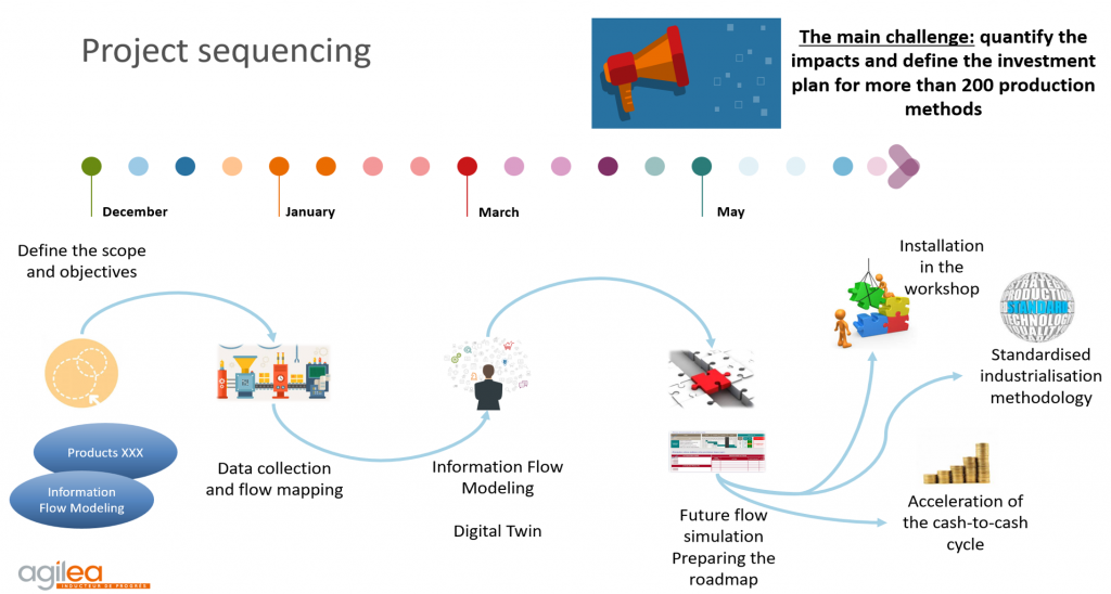
1) Achievements and results obtained
Data collection and mapping
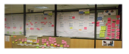
Figure 1: Value Stream Mapping (VSM)
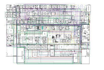
Figure 2: A Spaghetti Diagram
Use of Value Stream Mapping (VSM, figure 1) on well-known products in order to identify Non-Value Added (NVA) times.
Demonstrated level of complexity and a multitude of movements carried out (see Spaghetti Diagram, figure 2).
These 2 maps confirmed the need to use a simulation model to quantify future behaviour.
Process Mining and digital twin study
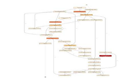
Figure 3: Process Mining report
– Average flow times exceeding 14 months for certain families.
– Many different operational sequences on so-called “standard” products (shown here, an example with 21 different operational sequences carried out on 22 MOs).
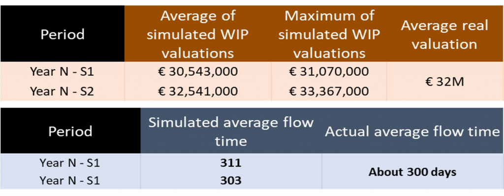
Figure 4: Simulated and actual results over the past year
A model that can be described as “calibrated” with very similar results in terms of load/capacity, flow time, valuated work in process and throughput (MOs completed over the past year: 1,227 / MOs completed in the model: 1,187).
Simulation of tomorrow’s flows and roadmap
From the simulation model representing the client’s environment, it is possible to project and quantify the years to come according to various scenarios.
The need for decision-making is more than justified by the graphs below which confirm a future with no changes made compared to the past year (an “explosion” of WIP and, consequently, flow times):
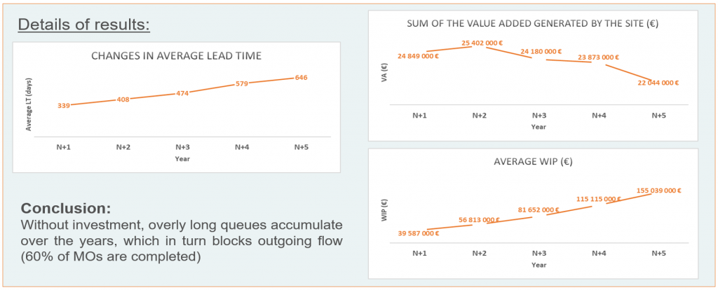
Figure 5: Results of the current system (“As-Is”) without change over the next 5 years
Compared to the initial findings of the projection of the model without modification, different improvement scenarios were defined with the client’s teams and evaluated. Below is a list of examples:
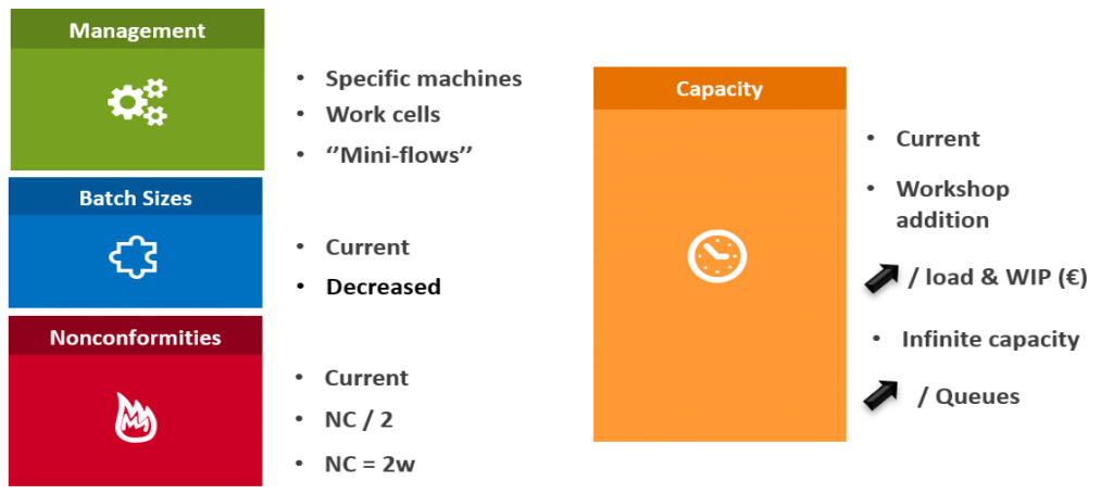
Figure 6: Examples of scenarios to be simulated
Presentation of simulated scenarios and impacts on the different indicators. Presentation of two example scenarios below, with:
– a “push flow” scenario (as currently used) with the needed investments, but with flow times which remain excessive in order for resources to have full loads (sometimes, even saturated).
– a scenario which uses queue management in order to promote the movement of flows and allow resources not to operate continually.
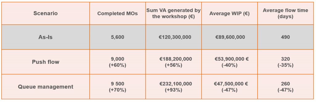
Figure 7: Results of the 2 scenarios compared to the projection of the current system (As-Is) over the 5-year period of simulation
The client defined the target (called the “To-Be” scenario) and now knows how much investment will need to be made in relation to this target, semester by semester:
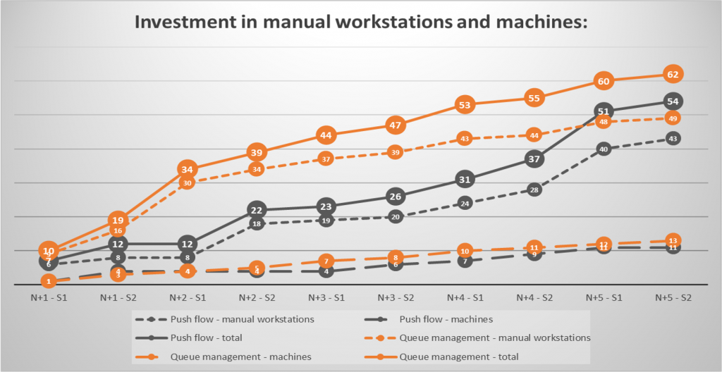
Figure 8: Recommended investments, semester by semester, according to each scenario
Project results
Difficulties encountered:
Data: The data collection stage was prolonged by the diversity of flows, the multitude of references and routings and the complex financial data.
Calibration: Given the challenges, a calibrated simulation model was needed (for obtaining the same results by replaying the past), with cost data and resource opening schedules that were initially erroneous (creation of non-existant queues in reality).
Management: The transition to queue management by agreeing not to continually use all of the means of production.
Results obtained
With the proposed evaluation, the client is able to imagine a workshop generating €50M of VA/year over a 5-year horizon, compared to the current €25M (for a constant amount of WIP).
The client better understands the behaviour of the company’s system, with the help of the analysis and the mapping of the different flows.
The client knows which resources to invest in, semester by semester, in relation to the defined target.
The client has a model that can be simulated again when demand assumptions change (quantity / product mix).
The client started queue management with one family of products: a reduction of more than half of the WIP for the flow times that were reduced by large proportions (as evaluated with the model).